

Value At Risk, abbreviated as VaR, and Expected Shortfall, abbreviated as ES are common terms that one would usually come across in measuring risk in finance.
We all want to make money but we don’t want to make rash decisions in doing so! In other words, we want to maximise our returns and minimise our risk. We intuitively understand these concepts, but how do we study these concepts from finance mathematically?
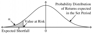
Let us say we have a probability distribution of our returns as follows. The y-axis is the probability while the x-axis is the returns. We see that our distribution has a peak at 0 and this tells us that the most likely outcome is that we neither make money nor lose money. It also tells us that we have a 50% probability to lose money and a 50% probability to make money. It also (if you’re a mathematician reading this, please pardon me for skipping the measure theory tit-bits!).
Now anyone would love to make a lot of money, but we notice from the distribution that this outcome, sadly, has a very low probability and is hence very unlikely! However, most people are more concerned with not losing their money compared to making a lot of money. Hence it is important to quantify how much money we stand to lose!
We first select and fix a significance level α or confidence level, (1-α)%. The more brave an individual is to face the risk of losing money, the lower is the α. Statisticians generally use an α=0.05 empirically.
Let us first understand the concept of Value at Risk or VaR.
Value At Risk is a measure of the potential losses that one could face. It answers the simple question, what is the minimum loss over the whole range of outcomes in the α% tail where I stand to lose? Graphically, it means the value at which the area under the curve sums up to α.
The VaR refers to a quantile. For an α = 0.05, we are interested in the 5% quantile of our returns—meaning that 95% of our returns are greater than the VaR, while 5% are to the left and hence lesser than the VaR. The smaller α is chosen, the further left on the distribution we are, and the more negative our VaR becomes.
Expected Shortfall or ES answers a different question:
What is the mean of the losses that I could face, over the tail that I stand to lose? Expected Shortfall Risk Measure, is a measure of the average losses over the α% losing tail.
Expected Shortfall, a concept used in the field of financial risk management takes the average of all the returns to the left of the VaR i.e. the returns which are less than the VaR. Since it is an expectation and is calculated by integrating over an entire region, it is a much more robust statistic compared to VaR which is just a single value.
Now, which one should we use for quantifying risk? Well, it depends! If you want to hate risks, use VaR. If you are a person who wants long-term returns, use ES!
Experimenting with data in R!
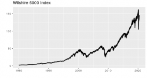
R is an awesome language for quantitative finance and computation risk assessment. Let us now apply what we learnt on a real data set on R! We choose the Wilshire 5000 dataset and our period of study. Don’t worry if you’ve never used R, I’ve added plenty of comments with the code so you can follow along and understand!
| # Import libraries and set seed library(quantmod); library(ggplot2); library(moments); library(MASS); library(metRology) set.seed(1) # Get Wilshire 5000 data wilshire <- getSymbols(Symbols = “WILL5000IND”, src = “FRED”, auto.assign = FALSE) wilshire <- na.omit(wilshire) wilshire <- wilshire[“1980-01-01/2020-06-01”]# Let us see what our data looks like!# Create time series plot of data ggplot(data = wilshire, aes(x = Index, y = WILL5000IND))+ geom_line(size = 1.0) + xlab(“”) + ylab(“”) + ggtitle(“Wilshire 5000 Index”) |
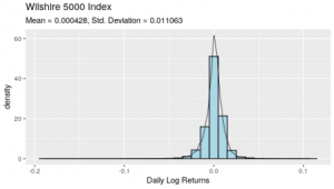
| log_returns <- diff(log(wilshire))[-1] # We calculate daily log returns instead of simple daily returns because# most of such data follow a right-skewed distribution which can be# approximated quite well by a log-normal distribution. A log-normal# distribution has a useful property that its log is normally distributed # which is quite easy to work with. mu <- round(mean(log_returns), 6) # Mean: 0.000428 sigma <- round(sd(log_returns), 6) # Standard Deviation: 0.011063 # Produce histogram of returns overlaid with a kernel density plot ggplot(data = log_returns, aes(x = WILL5000IND)) + geom_histogram(aes(y = ..density..), binwidth = 0.01, color = “black”, + geom_density(size = 0.3) + xlab(“Daily Log Returns”) + ggtitle(“Wilshire 5000 Index”, subtitle = “Mean = 0.000428, Std. Deviation = 0.011063”) |
| # Print skewness and kurtosis cat(“Skewness:”, skewness(log_returns), “Kurtosis:”, kurtosis(log_returns), sep = “\n”) We now estimate the VaR and ES using an empirical distribution- we simulate directly from our empirical distribution without making any assumptions about its shape. # Set a 95% confidence level alpha <- 0.05 # Random sample of 100,000 observations from the empirical distribution with replacement sample.empirical <- sample(as.vector(log_returns), 1000000, replace = TRUE) # Calculate VaR VaR.empirical <- round(quantile(log_returns, alpha), 6) # Calculate ES ES.empirical <- round(mean(sample.empirical[sample.empirical < VaR.empirical]), 6) # Print results cat(“Value at Risk:”, VaR.empirical, “Expected Shortfall:”, ES.empirical, sep = “\n”) And we now finally find the VaR and ES of the portfolio using the empirical distribution portfolio <- 1000 # Using VaR and ES from empirical distribution VaR.portfolio <- portfolio * (exp(VaR.empirical) – 1) ES.portfolio <- portfolio * (exp(ES.empirical) – 1) # Print results cat(“Value at Risk:”, VaR.portfolio, “Expected Shortfall:”, ES.portfolio, sep = “\n”) |
Hope this article gives you a comprehensive understanding of these two important statistics in measuring financial risk analytics!
References
Blog Published By: Mr. Ananyapam, Student Risk Committee Member