




Introduction
In layman’s terms, financial risk refers to the possibility of losing money on an investment or business operation. To manage this uncertainty, financial institutions, investors, and corporate risk managers rely heavily on financial risk measures — quantitative critical risk management tools designed to assess, monitor, and mitigate various types of financial risks.
Financial risk in transport infrastructure refers to the probability of encountering budget overruns or schedule delays during the planning, construction, or operational phases of a network. To control these highly capital-intensive uncertainties, project directors, government sponsors, and risk managers use quantitative risk analysis to track, and control financial exposure.
There are different categories of financial risks, including market risk (losses due to changes in market prices of materials), credit risk (default by suppliers/rolling stock contractors or joint-venture partners), operational risk (failures in internal processes, incorrect assumptions or cost estimates, geological barriers during tunnelling etc.,), model risks (selection of incorrect model for quantitative measures) and liquidity risk (inability to meet short-term financial demands). Each of these requires specific metrics to quantify exposure and potential loss.
Common financial risk measures include Value at Risk (VaR), which estimates the maximum loss over a specified period at a given confidence level; Expected Shortfall (ES), which looks at the average loss beyond the VaR threshold; and Standard Deviation, a basic measure of volatility. Other advanced techniques incorporate stress testing, scenario analysis, and credit scoring models.
In this article let’s discuss various measures for financial risk in the context of transport infrastructure in the United Kingdom (UK).
A. Mean and Standard Deviation
Mean: The mean represents the expected return (cost) of an asset or portfolio over a specific period that could impact and is typically calculated as the average of historical returns (costs).
Standard Deviation: The standard deviation measures the variability or volatility of returns, indicating how much they tend to deviate from the mean.
The application of the mean in transport infrastructure refers to the typical historical cost overruns encountered by the similar capital projects, while the standard deviation represents the volatility of the baseline cost overruns
| Paradox of cost estimation | Breaking the illusion |
| Project estimators often assemble highly detailed cost models supported by extensive documentation, vendor quotes, and rigorous logical justifications. This comprehensive backup material builds immense confidence among stakeholders, creating a powerful illusion that the project is insulated from significant financial variance and will conclude well within its budgeted limits. | The primary risk in cost estimation does not stem from a lack of diligence, but rather from the “Inside View” bias, where estimators mistake extreme line-item detail for accurate forecasting. Crucially, this perspective ignores “systematic friction”—the compounding effect of minor, unpredictable costs across project phases that inevitably drives projects over budget. |

| Optimism Bias | Reference Class Forecasting |
| The above behaviour is called “Optimism Bias (OB)”. It is the demonstrated systematic tendency for appraisers to be overly optimistic about key parameters.
The Green Book suggests that appraisers should make explicit, empirically based adjustments to the estimates of a project’s costs, benefits, and duration. |
Reference Class Forecasting (RCF) uses historical project data as a predictor of the uncertainty and risk of future projects, including the risk of optimism bias.
From the RCF data we can have an idea on how historically the cost overruns are occurring in the similar projects. With reference to a high level overview of OB data, in 2020, the cost overruns in Rail in the UK was 39%. |
With the help of Optimism guidance and Reference Class Forecasting, the risk managers can calculate the
- Mean i.e., where the centre of gravity sits for historical cost overruns and,
- Standard Deviation i.e., how volatile the cost overruns could be. For example, for a cost overrun of 39%, if there is a very low standard deviation that implies that most of the projects would be around the range of 39% cost overruns while if there is large standard deviation it implies that extreme longer tails (higher volatility)
Building an Efficient Frontier
Within financial risk, the concept of the efficient frontier, central to Modern Portfolio Theory (MPT), plays a critical role in selecting an optimised portfolio.
| Using Risk and Returns | Using Reference Class Forecasting (RCF) |
| The efficient frontier represents the set of portfolios that deliver the highest expected return for a given level of risk or, conversely, the lowest risk for a given return | Reference class Forecasting does not calculate financial returns, so for us to build an efficient frontier we may have to add little twists considering only cost overruns / schedule delays vs Standard Deviation as Risk. |

| Using Risk and Returns | Using Reference Class Forecasting (RCF) |
|
|
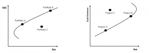
The above graphs are for illustrative purposes only. They do not reflect any actual data.
B. Value at Risk (VaR)
Value at Risk (VaR): It is one of the most widely used measures in financial risk management, serving as a benchmark to estimate potential losses within a portfolio or investment over a given period of time under normal market conditions. At its core, VaR provides an answer to a very practical question: “What is the worst expected loss that could occur over a specific time horizon at a given level of confidence?”
While calculating the historical mean provides a vital baseline estimate for potential cost overruns, relying on the average alone is statistically insufficient for final budgeting decisions. Knowing the mathematical average tells us where the historical centre of gravity lies, but it does not indicate the likelihood (at what confidence?) of our specific project landing near that number. Because capital infrastructure projects are highly volatile, we cannot assume our project will neatly match the mean. To establish a defensible budget, we must move beyond a single average value and determine the exact statistical confidence interval—quantifying the probability that our project will remain within a specified funding range.
In a standard trading style, VaR quantifies the maximum loss that is unlikely to be exceeded with a certain degree of confidence. For instance, if an analyst states that a portfolio has a one-month VaR of $1 million at a 95% confidence level, this can be interpreted to mean that, 19 out of 20 months, the portfolio is expected to either make a profit or, at worst, lose no more than $1 million. Conversely, in the remaining 5% of the time, losses could exceed this threshold, which reflects the tail risk that VaR does not capture.
Unlike a standard trading style VaR, which explicitly includes a specific time parameter, a Reference Class Forecasting (RCF) model calculates a maximum cost overrun at a chosen confidence level over the entire lifecycle of the project. To account for this missing temporal dimension and prevent eroded purchasing power, risk managers overlay macroeconomic inflation projections onto the RCF-adjusted cost overruns.
The concept of confidence level is central to understanding VaR. A confidence level represents the degree of statistical certainty with which the estimate is made. A 95% confidence level suggests a high probability that actual outcomes will remain within the projected limits, while a 95% level offers even greater assurance.
However, as the confidence level increases, the corresponding VaR estimate also rises because it must account for a broader range of adverse scenarios. This increase is driven by the dependence of VaR on the statistical Z-Score: the higher the confidence level, the larger the Z-Score, and thus, the higher the estimated potential loss. Importantly, VaR does not grow linearly with confidence but rather at an accelerating rate, since covering rarer extreme events requires progressively larger buffers.
Estimating VaR
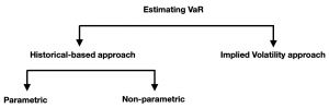
Below are the methods on how VaR is measured :
| Parametric VaR | Non-Parametric VaR | Implied Volatility |
| Parametric VaR, also known as delta-normal VaR, assumes that asset or portfolio returns follow a specific statistical distribution, most commonly the normal distribution | Non-parametric VaR avoids assumptions about the distribution of returns and instead relies on actual market data to model risk. The most common techniques include historical simulation, which uses past return data to directly determine the worst potential losses at a given confidence level | Implied volatility-based VaR relies on information embedded in option prices to estimate potential future risk. By applying option pricing models such as Black-Scholes, implied volatility is extracted from market option prices, which reflects the market’s own expectations of future volatility. |
Challenges in Estimating VaR
While VaR is a powerful tool, it is not without limitations. Two major categories of risk arise when applying it:
- Model Risk – This occurs when the assumptions underlying the chosen VaR model (such as distribution of returns, correlations, or volatility estimates) are flawed or unrealistic.
- Implementation Risk – Even with an appropriate model, errors can arise from the way it is applied in practice. These may include incorrect data inputs, computational mistakes, or misinterpretation of outputs, all of which could lead to misleading risk assessments.
In summary, Value at Risk is a practical and widely recognised method to measure and communicate potential losses with an associated probability of occurrence. It provides a common language for investors, risk managers, and regulators to discuss financial risk.
Expected Shortfall
In VaR Context – If a risk manager says, “The VaR is $10 billion at a 95% level of confidence, “then this translates to mean “under normal conditions, in 95% of confidence, we expect that the overall project lies with $10 billion.”
In Expected Shortfall Context – The 95% confidence level implies that there is a 5% chance where the project could exceed $10 billion
VaR vs ES – VaR is a quantile measure that provides a threshold of cost overruns but provides no information about the severity of the cost overruns beyond it. While ES is a tail measure that incorporates the extreme events.
VaR and ES vs project maturity
As we spoke about the importance of VaR and ES, now we need to understand when to calculate the model and when the outputs are valid. Initial Value at Risk (VaR) and Expected Shortfall (ES) outputs calculated at a project’s launch are merely baseline snapshots; relying on them as static metrics is a severe project flaw.
With reference to Project Management Institute (PMI)’s Risk Burnout chart, the risks and uncertainties over the project life reduces as the project becomes clearer and the assumptions would crystallise as we progress through the project.
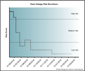
Source: Risk Burndown Charts
The project lifecycle for capital transport infrastructure projects is generally divided into 3 phases. For example, rail infrastructure is categorised as Strategic Outline Business Case (SOBC), Outline Business Case (OBC) and Full Business Case (FBC) phases. As the project progresses through SOBC-OBC-FBC the design, cost assumptions, estimates become more clearer and this helps as a valuable input to the model.
Computing VaR and Expected Shortfall using Historical Simulations
Historical simulation methods can be used to calculate both VaR and expected shortfall. Below are the high-level steps to calculate transport risk based on historical simulations for transport infrastructure projects:
Stage 1: Get the base line RCF data ready
- Determine the nature of the project
- Identify the stage of the scheme development
- Apply the recommended uplift factors to the base capital cost estimate
Stage 2: Quantified Risk Simulations on Project Risk Registers
- Utilize @RISK to run Monte Carlo simulations on the explicit project risk register and value management register to calculate bottom-up VaR and Expected Shortfall metrics.
Stage 3: Reconciliation
- Reconcile the @RISK simulation outputs against the Stage empirical uplifts to avoid risk double-counting, ensuring a compliant risk-adjusted budget.
C. Coherent Risk Measures
Coherent Risk Measures are a class of risk measures in financial risk management that satisfy a set of desirable properties, ensuring they provide a consistent, logical, and reliable assessment of risk. A risk measure is considered coherent if it satisfies the following properties:
- Monotonicity: If a portfolio A is riskier than B, then the risk measure of A should be greater than B
- Subadditivity: Risk of a combined portfolio should not exceed the sum of the risks of individual portfolios
- Positive Homogeneity: If a portfolio is scaled by a positive factor, the risk measure should scale by the same factor
- Translation Invariance: If a risk-free asset is added to a portfolio, the risk measure should decrease by an amount equal to the value of the risk-free asset.
VaR and Expected Shortfall are the examples of coherent risk measures
D. Stress Testing
Stress testing is a critical enterprise risk management tool used to evaluate organisational resilience, and the financial resilience of capital projects under extreme but plausible economic and delivery conditions. A key motivation for stress testing stems from the observation that during major macroeconomic shocks or systemic industry failures, correlations between project risks rise sharply.
There are two main approaches to conduct stress testing:
| Historical Crisis | Hypothetical or pre-determined stress scenarios |
| Risk managers apply cost overruns and contractor defaults from past crises (like COVID-19 or the 2008 crash) to current projects. This tests pipeline resilience against real-world systemic shocks. | Risk managers simulate forward-looking, extreme shocks like hyperinflation, extended approval delays, and tier-1 contractor insolvencies etc., This checks project vulnerability against unprecedented market threats. |
Now the main question is – “Are extreme economic crises not already covered in Reference Class Forecasting (RCF) uplifts? Since RCF captures decades of actual cost overruns from similar historical projects, shouldn’t it already account for these events?”
Below is the key difference between the RCF uplifts vs the stress testing:
RCF: This provides us the aggregated and blended history of variances across similar projects for the past several years. This will provide us the “Realistic Budget”
Stress test: This is very isolated and specific history covering 1 or 2 specific history market failures. This will check the catastrophic insolvency or funding gaps. This will act as a “Conservative Reserve” for the project
E. Operational and Non-Financial Risk Measures
The other set of Risk measures that captures the failures in people, process and procedures etc. These operational risk management measures include:
- Key Risk Indicators (KRI’s)
- KRIs are measurable metrics that serve as early warning signals for potential risk events or vulnerabilities in operations.
- Examples include Number of failed transactions, frequency of IT system outages, rising staff turnover, number of cybersecurity breaches, percentage of overdue reconciliations etc.,
- KRIs support risk appetite frameworks by tracking whether risk exposure is within tolerances.
- Risk Control Self-Assessment (RCSA)
- A structured qualitative process where business units identify and evaluate their own risk exposures, as well as the effectiveness of controls in place.
- RCSA encourages ownership of risks within each business function
- It highlights areas needing stronger controls, training, or automation.
- Business Continuity and Resilience Planning
- A set of policies, procedures, and stress tests designed to ensure that critical business operations can continue during and after disruptions.
- Business Continuity Planning and Resilience Planning revolves around IT failures, natural disasters, cyber incidents, pandemic shocks, supplier breakdowns, and other external disruptions.
The author of this article is Mr. Kishore Varanasi, IRMCert®. The author confirms that this article is original and has not been copied, reproduced, or derived from another author’s work, except for appropriately cited third-party references used for research purposes.
References
Department for Transport. (2025). TAG Unit A1.2 scheme costs. https://www.gov.uk/transport-analysis-guidance-tag
Hopkin, Paul. (2018). Fundamentals of risk management: understanding evaluating and implementing effective risk management, 5th ed. (5). : Kogan Page.
Risk Burndown Chart – Project Management Institute
UK GOVERNMENT. (2026). THE GREEN BOOK [Report].
https://assets.publishing.service.gov.uk/media/698dbcd17da91680ad7f4308/The_Green_Book_2026.pdf
FAQs:
1. What is Value at Risk (VaR)?
Value at Risk (VaR) is one of the most widely used measures in financial risk management, serving as a benchmark to estimate potential losses within a portfolio or investment over a given period of time under normal market conditions.
2. What does “expected shortfall” mean?
While VaR is a quantile measure that provides a threshold of cost overruns but provides no information about the severity of the cost overruns beyond it, Expected Shortfall is a tail measure that incorporates the extreme events.
3. What causes cost overruns in projects?
The primary risk in cost estimation does not stem from a lack of diligence, but rather from the “Inside View” bias, where estimators mistake extreme line-item detail for accurate forecasting. Crucially, this perspective ignores “systematic friction”—the compounding effect of minor, unpredictable costs across project phases that inevitably drives projects over budget.
4. How to quantify financial risk?
Common financial risk measures include Value at Risk (VaR), which estimates the maximum loss over a specified period at a given confidence level; Expected Shortfall (ES), which looks at the average loss beyond the VaR threshold; and Standard Deviation, a basic measure of volatility. Other advanced techniques incorporate stress testing, scenario analysis, and credit scoring models.
5. How can transport infrastructure projects improve financial resilience?
Transport infrastructure projects can improve financial resilience by adopting the following measures –
- Stress testing – Stress testing is a critical risk management tool used to evaluate the financial resilience of capital projects under extreme but plausible economic and delivery conditions.
- Tracking Key Risk Indicators (KRI’s) – KRIs are measurable metrics that serve as early warning signals for potential risk events or vulnerabilities in operations. Examples include Number of failed transactions, frequency of IT system outages, rising staff turnover, number of cybersecurity breaches, percentage of overdue reconciliations etc. KRIs support risk appetite frameworks by tracking whether risk exposure is within tolerances.
- Conducting Risk Control Self-Assessment (RCSA) – Risk Control Self-Assessment is a structured qualitative process where business units identify and evaluate their own risk exposures, as well as the effectiveness of controls in place. RCSA encourages ownership of risks within each business function. It highlights areas needing stronger controls, training, or automation.
- Business Continuity and Resilience Planning – A set of policies, procedures, and stress tests designed to ensure that critical business operations can continue during and after disruptions. Business Continuity and Resilience Planning revolves around IT failures, natural disasters, cyber incidents, pandemic shocks, supplier breakdowns, and other external disruptions.